You have a long list that you want to put in an XML format. This tutorial will show you a quick way to do it with Microsoft Excel.
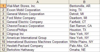
For this example, I have a list of the Fortune 100 companies and their locations. You can download (Right-click and “Save As”) the list and following along the tutorial.

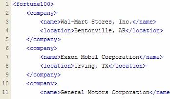
I want to take this list and put it in the following XML format:
<fortune100>

<company>

<name></name>

<location></location>

</company>

</fortune100>
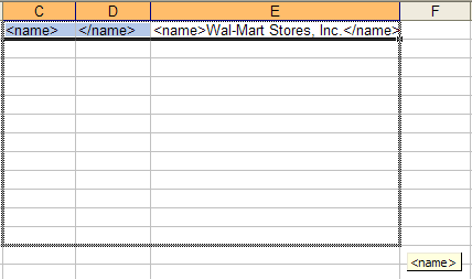
In two empty columns, I’m going to put the opening and closing tags for the names of the companies.

In a third empty column, I’m going to put in an Excel formula that will display Wal-Mart Stores, Inc. inside thetags. The formula I used is =C1&A1&D1. In layman’s terms, this formula is going to display the contents of cells C1, A1, and D1 in that order.
The result of the formulas is as follows.

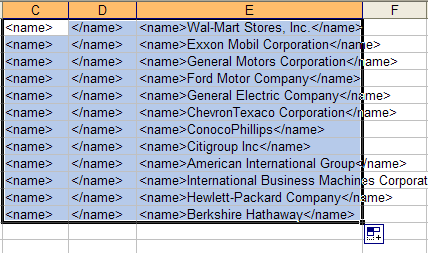
The next thing we want to do is create the same formula for the entire list of companies. By selecting cells C1, D1, and E1, and then left-clicking the bottom right-hand corner of cell E1, I can drag my mouse down and apply the contents/formulas of the selected cells to the cells below them.


Do this for your entire list.
You’re not done yet. Since column E is dynamically generated from a formula, you need to get actual list of what the formulas are producing.
Select column E and copy it. With Column E still selected, click the arrow to the right of the Paste icon on the toolbar and select “Values”.
This will paste the actual values of the formulas into the column. You can then cut-n-paste this column into whatever editor you use to edit XML files.
Column C and D can be deleted. Repeat this process for the location and you’re done applying XML formatting using Excel.

Thanks to Steve DiBello for showing me this quick and dirty trick.
Advanced Method
Patrick H contributed the following quicker method:
="<company><name>"&A5&"</name><location>"&B5&"</location></company>"


